
T1- and ECV-mapping in the heart:estimation of error maps and the influence ofnoise on precision
Peter Kellman
Andrew E. Arai
Hui Xue


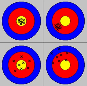
Precise
Imprecise
(reproducibility
error)
Accurate
Inaccurate
(systematic error)
Accuracy vs Precision:
•Calculation or T1-error from fit residuals
•Formulation for parameter errors
•PSIR fitting
•Robust variance estimates
•Validation of precision estimate
•Numerical simulation (Monte-Carlo)
•Phantom measurements (repeated trials)
•In-vivo results
•Variation with surface coil (SNR)
•Statistical significance of elevated T1 findings
•ROI vs pixel-wise statistics
•Motion related errors
•Protocol comparisons from precision standpoint
Outline
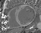
MOLLI Image Acquisition
Messroghli DR, et al. Modified Look-Locker inversion recovery (MOLLI) for high-resolution T1 mapping of theheart. Magn Reson Med. 2004;52(1):141-6.
Messroghli DR, et al. Optimization and validation of a fully-integrated pulse sequence for modified look-lockerinversion-recovery (MOLLI) T1 mapping of the heart. J Magn Reson Imaging 2007;26:1081-6.
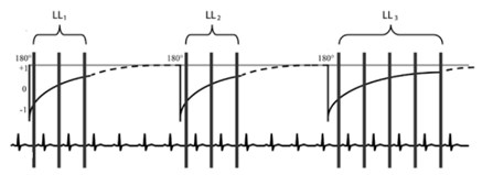
3(3)3(3)5
protocol

0
0
1
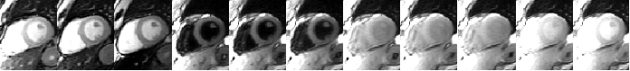
TI (ms)
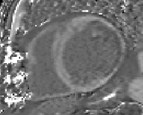
pixelwise fit
T1 map
0
500
1000
1500
2000
2500
3000
3500
4000
4500
5000
-100
-80
-60
-40
-20
0
20
40
60
80
100
PSIR Fit
Magnitude IR Fit
inversion time (ms)
MF-MagIR
PSIR
Xue H, et al. Phase-sensitive inversion recovery for myocardial T1 mapping with motioncorrection and parametric fitting. Magn Reson Med. 2012
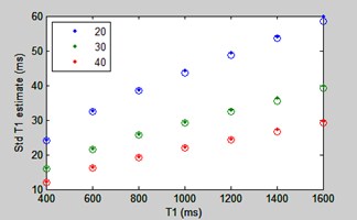
200
400
600
800
1000
1200
1400
1600
1800
0
20
40
60
80
100
120
140
T1 (ms)
Std T1 estimate (ms)
Sampling = [5 3] Heart rate = 60 TImin (ms) = 105 TIshift (ms) = 80
3 parameter simplex fit
10
20
30
PSIR
MF-MagIR
PSIR:3-parameter fit
Magn IR:3-parameter fit + zero crossing
PSIR reconstruction improve fitsresidual errors have normal distribution
Calculation of T1 error from fit residuals
3-parameter
robust fit to PSIR data
S = A – B exp(-TI/T1*)
Signal samples, S(i)
Inversion times, TI(i)
residuals, (i)
robust estimation of
standard deviation
calculate parameter
covariance matrix
Std dev,
Fit parameters, A, B, T1*
Inversion times, TI(i)
Robust estimation of standard deviationMedian Absolute Deviation (MAD)
Robust fit using iterative re-weighting
reduced weighting of outliers
Compute noise standard deviation from residual errors
estimated noise std
i = (fit – meas) residuals
Drop (p – 1) lowest residual values, p = 3 = number of fit parameters
ri = residuals for highest n-p+1 values of i
Compute median absolute deviation estimate
= median(abs(ri))/0.6745 (for Normal distribution)
*Hill RW & Holland PW, Two Robust Alternatives to Least Squares Regression. J. AmericanStatistical Assoc. 72:828-833.
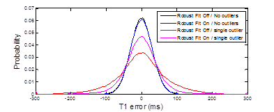
-----------------------------------
Single 6 SD outlier at random TI
T1 = 1100, SNR = 30, 5-3 sampling
-----------------------------------
Standard(without outliers):
true: 30.34 estimated: 31.57
Robust(without outliers):
true: 31.32 estimated: 30.92
Standard(with outliers):
true: 71.66 estimated: 64.75
Robust(with outliers):
true: 57.21 estimated: 55.70
-----------------------------------
Calculation of T1 from fit residuals
Alper JS, et al, J Phy Chem 1990. 94, 4747-51.
3 parameter signal model
Partial derivatives
Hessian matrix
Covariance matrix


Monte-carlo numerical validationT1 vs T1 & SNR
MOLLI 5(3)3 protocol
actual
estimated
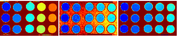
Phantom validation200 trials
T1-map
Calculated SD Map
200 trials
Estimated SD Map
(average of 200)
0
20
40
60
1000
2000
0
T1(ms)
T1(ms)
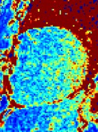
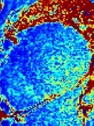
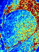
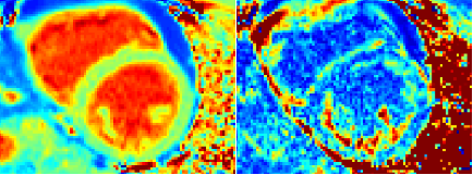
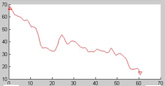
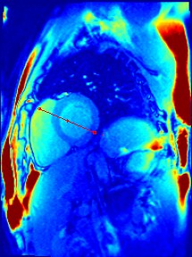
Dependence of T1 error with SNRresulting from drop off of surface coil sensitivity
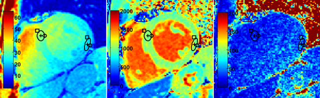
SNR map
T1-map
T1-std map
SD=41.8ms
SNR=32.1
T1=1012ms
SD=25.0ms
SNR=20.9
T1=1026ms
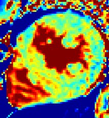
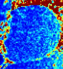
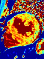
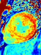
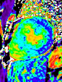
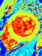
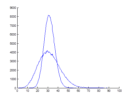
Subject with myocarditissignificant sub-epicardial focal elevation of T1
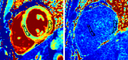
mean=1098 ms
mean=995 ms
SD= 43 ms
T1 elevated 103 ms ≈ 2.5 SD on a pixel-wise basis
ROI size = 48 pixels (≈ 19 independent pixels)
SD ≈ 43/sqrt(19) ≈ 10 ms on ROI basis (10 SD > septal ROI)
T1 in Septal Region is elevated 84 ms
(2.1 SD on pixel-wise basis; ≈ 16 SD on ROI basis
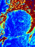
= 36 ms
mean= 1170 ms
mean= 1086 ms
= 42 ms
T1-map
800
900
1000
1100
1200
1300
1400
0
20
40
60
80
100
120
140
160
180
200
error-map
ms
ms
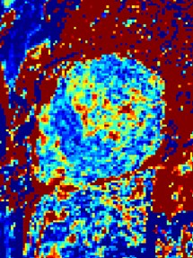
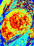
Subject with HCMAbility to detect subtle focal variations in T1
0
10
20
30
40
50
60
70
80
90
100
200
250
300
350
400
450
500
550
600
0
10
20
30
40
50
60
70
80
90
100
T1 (ms)
SD (ms)
= 36 ms
= 42 ms
mean= 1170 ms
mean= 1086 ms
700
800
900
1000
1100
1200
1300
E05411
0
0.02
0.04
0.06
0.08
0.1
0.12
0.14
0.16
0.18
0.2
0.5
0.6
0.7
0.8
0.9
1
1.1
1.2
1.3
1.4
1.5
1
1.2
1.4
1.6
1.8
2
2.2
2.4
2.6
2.8
3
0
0.02
0.04
0.06
0.08
0.1
0.12
0.14
0.16
0.18
0.2
R1 (Hz)
SD (Hz)
Reformulated for R1
0
10
20
30
40
50
60
70
80
90
100
0
0.5
1
1.5
2
2.5
3
3.5
4
4.5
5
ECV (%)
SD (%)
septal ROI:34.8 ± 1.0% (m ± SD)
lateral wall ROI:26.2 ± 1.2%.
1
1
1
1
1
1
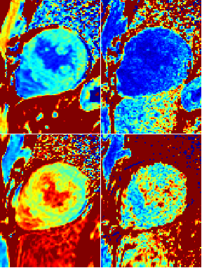
MOLLI
5(3s)3
SASHA
1-10
2-param fit
SASHA
1-10
3-param fit
= 42 ms
= 59 ms
= 133 ms

mean= 1038 ms
mean = 1151
mean= 1180
0
50
100
150
200
0
500
1000
1500
2000
T1 (ms)
T1 (ms)
Example: invivo comparison of techniques
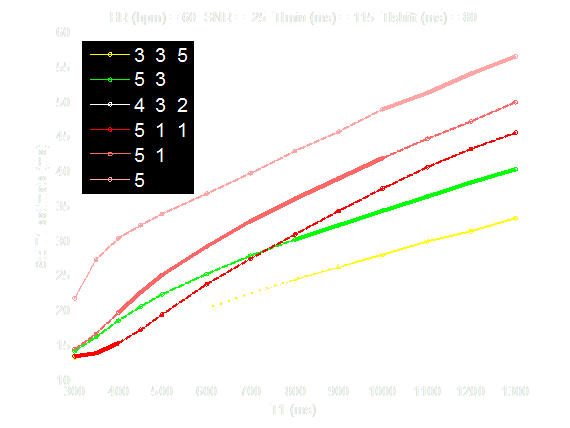
Precision:MOLLI sampling schemes
Original
MOLLI
Protocol
3-3-5
ShMOLLI
Protocol
5-3
4-3-2
5-0
5-1
5-1-1
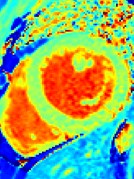
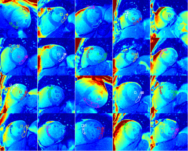
SD maps serve as an indication of T1-map quality
Uncorrected motion errorsrecognized by appearance of structure
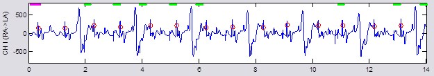
Patient with PVCs results in cardiac motion
•Estimate of T1 measurement error (SD maps)
•Robust unbiased formulation
•Implemented on-line scanner
•Useful for assessing quality of maps
•Useful for determining statistical significance
•Useful for comparison of techniques andprotocol optimization
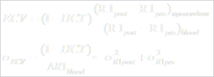
•formulation extended to R1=1/T1 to calculateSD maps for extracellular volume (ECV)fraction
Summary
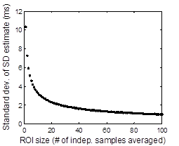
N = 4 pixels
N = 1 pixel
(no averaging)
Std deviation of SD estimate5(3)3 protocol with 8 inversion times
0
20
40
60
80
100
120
SNR32 channel cardiac array
0
20
40
60
80
100
120
septum
LV blood
lateral
wall
256x144
1.4x1.9 mm2
SNRseptum = 43 ± 11
SNRlateral = 22.8 ± 4.3
(N=20 subjects)